
Investigating crashes using API data
The Jupyter notebook can be accessed here
A number of factors can increase the chances of a car crash occurring - for instance: weather, drink-driving or time of day. In this project, I set out to collect data from the web in order to understand the circumstances surrounding car crashes in the state of Maryland, U.S. The crash data was taken from the U.S. website: data.gov.
- First of all, the Foursquare API is used to collect data about the number of bars within in a certain radius in each County, in order to see if the prevalence of drinking might have an influence on the accident rate.
- Second of all, the Google Maps API is used to determine the coordinates of each county, then the coordinates are used to request the weather conditions at the time of the accident from the DarkSky API.
- Finally, the coordinates of the accidents themselves are obtained and plotted on a map using the Google Map Plotter.
Data
The data for this exercise can be found here.
I will now add the dataset to a Pandas dataframe.
import pandas as pd
mypath = "./"
data = pd.read_csv(mypath + "2012_Vehicle_Collisions_Investigated_by_State_Police.csv",
                   parse_dates=[["ACC_DATE", "ACC_TIME"]])
data["MONTH"] = data.ACC_DATE_ACC_TIME.dt.month
data.dropna(subset=["COUNTY_NAME"], inplace=True) #get rid of empty counties
Here is what our dataframe looks like.
data.head()
| ACC_DATE_ACC_TIME | CASE_NUMBER | BARRACK | ACC_TIME_CODE | DAY_OF_WEEK | ROAD | INTERSECT_ROAD | DIST_FROM_INTERSECT | DIST_DIRECTION | CITY_NAME | COUNTY_CODE | COUNTY_NAME | VEHICLE_COUNT | PROP_DEST | INJURY | COLLISION_WITH_1 | COLLISION_WITH_2 | MONTH | |
|---|---|---|---|---|---|---|---|---|---|---|---|---|---|---|---|---|---|---|
| 0 | 2012-01-01 02:01:00 | 1363000002 | Rockville | 1 | SUNDAY | IS 00495 CAPITAL BELTWAY | IS 00270 EISENHOWER MEMORIAL | 0.00 | U | Not Applicable | 15.0 | Montgomery | 2.0 | YES | NO | VEH | OTHER-COLLISION | 1 |
| 1 | 2012-01-01 18:01:00 | 1296000023 | Berlin | 5 | SUNDAY | MD 00090 OCEAN CITY EXPWY | CO 00220 ST MARTINS NECK RD | 0.25 | W | Not Applicable | 23.0 | Worcester | 1.0 | YES | NO | FIXED OBJ | OTHER-COLLISION | 1 |
| 2 | 2012-01-01 07:01:00 | 1283000016 | Prince Frederick | 2 | SUNDAY | MD 00765 MAIN ST | CO 00208 DUKE ST | 100.00 | S | Not Applicable | 4.0 | Calvert | 1.0 | YES | NO | FIXED OBJ | FIXED OBJ | 1 |
| 3 | 2012-01-01 00:01:00 | 1282000006 | Leonardtown | 1 | SUNDAY | MD 00944 MERVELL DEAN RD | MD 00235 THREE NOTCH RD | 10.00 | E | Not Applicable | 18.0 | St. Marys | 1.0 | YES | NO | FIXED OBJ | OTHER-COLLISION | 1 |
| 4 | 2012-01-01 01:01:00 | 1267000007 | Essex | 1 | SUNDAY | IS 00695 BALTO BELTWAY | IS 00083 HARRISBURG EXPWY | 100.00 | S | Not Applicable | 3.0 | Baltimore | 2.0 | YES | NO | VEH | OTHER-COLLISION | 1 |
I am now curious about the counties in Maryland, so I will take a look.
data.COUNTY_NAME.unique()
array(['Montgomery', 'Worcester', 'Calvert', 'St. Marys', 'Baltimore',
       'Prince Georges', 'Anne Arundel', 'Cecil', 'Charles', 'Carroll',
       'Harford', 'Frederick', 'Howard', 'Allegany', 'Garrett', 'Kent',
       'Queen Annes', 'Washington', 'Somerset', 'Wicomico', 'Talbot',
       'Caroline', 'Dorchester', 'Not Applicable', 'Unknown',
       'Baltimore City'], dtype=object)
Google Maps API
I will now setup the google maps API, which will come in handy later on.
from googlemaps.exceptions import TransportError
import googlemaps
from googlemaps.exceptions import HTTPError
gmaps = googlemaps.Client(key=os.environ["[YOUR API KEY HERE]"])
county_names = list(set(data.COUNTY_NAME.unique()))
Foursquare API
I will now use the Foursquare API to collect data in the vicinity of the coordinates give for each county. Ultimately, I want to know how many bars there are within a radius of 5 km.
Foursquare API documentation is here
The objective for this part are:
- Start a foursquare application and get your keys.
- For each crash, pull number of of bars (category “Nightlife”) in 5km radius.
- Find a relationship between number of bars in the area and severity of the crash.
#set the keys
foursquare_id = '[YOUR API KEY HERE]'
foursquare_secret = "YOUR SECRET CODE HERE"
#install and load the library
from foursquare import Foursquare
Now we need to set up the client in order to make calls to the API.
client = Foursquare(client_id = foursquare_id,
                   client_secret = foursquare_secret)
We will loop through the counties and obtain the number of bars within a 5km radius (up to a maximum of 50 bars). If the call quota is exceeded, then the operation will be paused for one hour to allow it to reset.
number_of_bars = {}
for county in county_names:
    try:
        response = client.venues.search({'near': county,
                                         'limit': 50,
                                         'intent': 'browse',
                                        'radius': 5000,
                                        'units': 'si',
                                        'categoryId': '4d4b7105d754a06376d81259'})
        number_of_bars[county] = len(response['venues'])
    except Exception as e:
        print (e)
        if e == "Quota exceeded":
            print ("exceeded quota: waiting for an hour")
            time.sleep(3600)
        number_of_bars[county] = -1
Number of bars:
{'Allegany': 30,
 'Anne Arundel': 49,
 'Baltimore': 50,
 'Baltimore City': 50,
 'Calvert': 0,
 'Caroline': 6,
 'Carroll': 22,
 'Cecil': 28,
 'Charles': 13,
 'Dorchester': 22,
 'Frederick': 35,
 'Garrett': 12,
 'Harford': 2,
 'Howard': 9,
 'Kent': 19,
 'Montgomery': 50,
 'Not Applicable': -1,
 'Prince Georges': 29,
 'Queen Annes': 8,
 'Somerset': 41,
 'St. Marys': 13,
 'Talbot': 3,
 'Unknown': 0,
 'Washington': 50,
 'Wicomico': 50,
 'Worcester': 36}
We need to select a target variable. I will choose the ‘INJURY’ column, because this is a straightforward way to judge the severity of the crash.
# Converting injuries to a binary mapping to judge severity
data_df['severity'] = data_df['INJURY'].map({'YES':1, 'NO':0})
I will now create a new dataframe for my features and encode each feature into categoric variables.
from sklearn.preprocessing import LabelEncoder
le = LabelEncoder()
# crash severity
feature_df = pd.DataFrame()
feature_df['id'] = data_df['CASE_NUMBER']
feature_df['Time'] = data_df['ACC_TIME_CODE']
feature_df['Day'] = le.fit_transform(data_df['DAY_OF_WEEK'])
feature_df['Vehicles'] = data_df['VEHICLE_COUNT'].fillna(0)
feature_df['One hit'] = le.fit_transform(data_df['COLLISION_WITH_1'])
feature_df['Tws hits'] = le.fit_transform(data_df['COLLISION_WITH_2'])
feature_df['Bars'] = data_df['num_bars']
I need to make sure that there are no missing values, otherwise I can expect problems in the next step.
# Let's make sure that there are no missing values because they will cause the algorithm to crash
feature_df.isna().sum()
I will now use the Scikit-learn random forest classifier to fit a model and use that model to determine the importance of each feature.
from sklearn.ensemble import RandomForestClassifier
# Sets up a classifier and fits a model to all features of the dataset
clf = RandomForestClassifier(n_estimators=150, max_depth=8, min_samples_leaf=4, max_features=0.2, n_jobs=-1, random_state=0)
clf.fit(feature_df.drop(['id'],axis=1), data_df['severity'])
# We need a list of features as well
features = feature_df.drop(['id'],axis=1).columns.values
print("--- COMPLETE ---")
Using the following code from Anisotropic’s kernal (https://www.kaggle.com/arthurtok/interactive-porto-insights-a-plot-ly-tutorial), we can use Plotly to create a nice horizontal bar chart for visualising the ranking of the most important features for determing the severity of crash.
import plotly.offline as py
py.init_notebook_mode(connected=True)
import plotly.graph_objs as go
import plotly.tools as tls

x, y = (list(x) for x in zip(*sorted(zip(clf.feature_importances_, features),
                                                            reverse = False)))
trace2 = go.Bar(
    x=x ,
    y=y,
    marker=dict(
        color=x,
        colorscale = 'Viridis',
        reversescale = True
    ),
    name='Random Forest Feature importance',
    orientation='v',
)

layout = dict(
    title='Ranking of most influential features',
     width = 900, height = 1500,
    yaxis=dict(
        showgrid=False,
        showline=False,
        showticklabels=True,
    ))

fig1 = go.Figure(data=[trace2])
fig1['layout'].update(layout)
py.iplot(fig1, filename='plots')
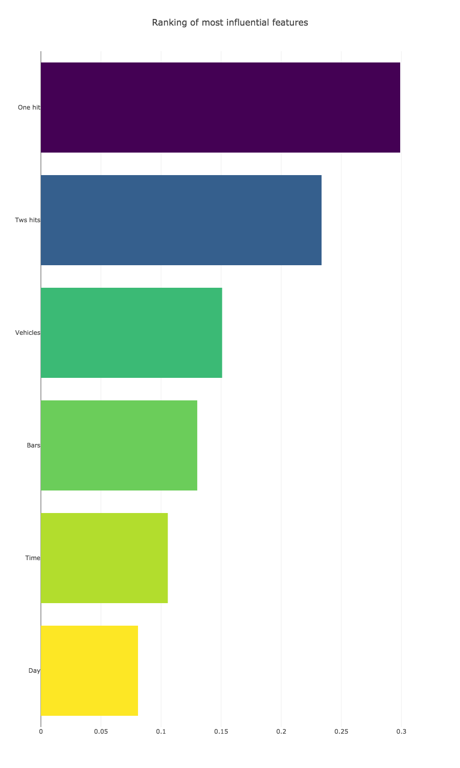
As we can see here, the number of bars does not have the biggest influence; however, it has a bigger influence than the time the accident occurred or the day of the week.
DarkSky API
This time I will make calls to the DarkSky API for each crash in a sample set (limited call quota) to get weather information at the time of the accident.
DarkSky API documentation is here
The time needs to be converted to unix in order for the DarkSky API to recognise it.
def time_to_unix(t):
    return time.mktime(t.timetuple())

# changing to unix time
data_sample_df = data_df.sample(n=1000, random_state=0)
data_sample_df['UNIX_TIME'] = data_sample_df['ACC_DATE_ACC_TIME'].apply(time_to_unix).astype(int)
We now need to get the latitude and longitude for each county from the Google Maps API in order to get the weather information at the approximate location of each crash. We can makes calls to the Google Maps API to do this.
def get_lat_lng(data, state, place_col):
    places = list(set(data[place_col].unique()))

    geo_dict = {'place':[], 'lat':[], 'lng':[]}
    for i in range(len(places)):
        place = places[i] + ', ' + state
        try:
            lat = gmaps.geocode(place)[0]['geometry']['location']['lat']
            lng = gmaps.geocode(place)[0]['geometry']['location']['lng']
            geo_dict['place'].append(places[i])
            geo_dict['lat'].append(lat)
            geo_dict['lng'].append(lng)
        except:
            geo_dict['place'].append(None)
            geo_dict['lat'].append(None)
            geo_dict['lng'].append(None)

    geo_df = pd.DataFrame(geo_dict)
    return pd.merge(data, geo_df, left_on='COUNTY_NAME', right_on='place', how='left')

data_sample_geo_df = get_lat_lng(data_sample_df, 'Maryland', 'COUNTY_NAME')
We need to specify our own unique API key.
# Once you have signed up on DarkSky.net, you will be given an API key, which you need to insert here.
api_key = "[YOUR API KEY HERE]"
The next step is to make calls (requests) to the API for each of the crash instances in our sample. I am simply appending each entry into a dictionary with the place, coordinates, time and returned results.
import requests
import time

weather_data = {'place': [], 'lat': [], 'lng': [], 'time': [], 'result': []}

for crash in data_sample_geo_df.iterrows():
    place = crash[1]['COUNTY_NAME']
    lat = crash[1]['lat']
    lng = crash[1]['lng']
    t = crash[1]['UNIX_TIME']
    # https://api.darksky.net/forecast/[key]/[latitude],[longitude],[time]
    request = 'https://api.darksky.net/forecast/' + api_key + '/' + str(lat) + ',' + str(lng) + ',' + str(t)

    try:
        result = requests.get(request).content

        weather_data['place'].append(place)
        weather_data['lat'].append(lat)
        weather_data['lng'].append(lng)
        weather_data['time'].append(t)
        weather_data['result'].append(result)
    except Exception as e:
        print(e)
        weather_data['place'].append('')
        weather_data['lat'].append('')
        weather_data['lng'].append('')
        weather_data['time'].append('')
        weather_data['result'].append('')
Now I will concatenate the results into the sample dataframe that contains information about each crash, as well as the GPS coordinates.
weather_df = pd.concat([data_sample_geo_df[['CASE_NUMBER']], pd.DataFrame(weather_data).reset_index(drop=True)], axis=1)
# I like to save results like these in a CSV file, because there is a limit on the number of API calls
weather_df.to_csv('weather-data.csv')
After going through one of the JSON files that was returned to me, I found the section that I want (“currently”). It contains the overall weather conditions, precipitation type (if any) and most importantly, the chance of rain. If the chance is greater than 50%, then I am satisfied that if was raining at the time for the sake of this exercise.
import json

def extract_data(x):
    try:
        d = json.loads(x)
        res = d['currently']['precipProbability']
    except Exception as e:
        print (e)
        res = ''
    return res

weather_df['precipProb'] = weather_df['result'].apply(extract_data)
Expecting value: line 1 column 1 (char 0)
One line failed, so I will insert a zero.
weather_df['precipProb'] = weather_df['precipProb'].replace('', 0)
Now I should merge the original sample dataset and the weather data.
df_final = data_sample_df.merge(weather_df, left_on='CASE_NUMBER', right_on='CASE_NUMBER', how='outer')
I can use the Pointbiserialr tool from Scipy stats to calculate the correlation and the p-value between the binary values of the ‘severity’ and the continuous values of the ‘precipProb’ (probability of precipitation) column.
from scipy.stats import pointbiserialr

corr = pointbiserialr(df_final['severity'], df_final['precipProb'])
corr
PointbiserialrResult(correlation=-0.01817849772457154, pvalue=0.56584394823957873)
We see here that the correlation is not strong at all, only -0.018, with a p-value greater than 0.5. This is a surprising result, as we cannot say that rain causes a statistically significant increase in accidents.
Adding weather to feature set
The precipitation probability feature can be included in a new feature table, along with the other features we used before.
from sklearn.preprocessing import LabelEncoder
le = LabelEncoder()
# crash severity
feature_df = pd.DataFrame()
feature_df['id'] = df_final['CASE_NUMBER']
feature_df['Time'] = df_final['ACC_TIME_CODE']
feature_df['Day'] = le.fit_transform(df_final['DAY_OF_WEEK'])
feature_df['Vehicles'] = df_final['VEHICLE_COUNT'].fillna(0)
feature_df['One hit'] = le.fit_transform(df_final['COLLISION_WITH_1'])
feature_df['Tws hits'] = le.fit_transform(df_final['COLLISION_WITH_2'])
feature_df['Bars'] = df_final['num_bars']
feature_df['rain'] = df_final['precipProb']

feature_df.head()
| id | Time | Day | Vehicles | One hit | Tws hits | Bars | rain | |
|---|---|---|---|---|---|---|---|---|
| 0 | 1251037421 | 3 | 6 | 2.0 | 6 | 2 | 35 | 0.0 |
| 1 | 1251029176 | 6 | 1 | 2.0 | 6 | 2 | 35 | 0.0 |
| 2 | 1280008862 | 5 | 0 | 2.0 | 6 | 4 | 8 | 0.0 |
| 3 | 1294006103 | 2 | 4 | 1.0 | 4 | 0 | 12 | 0.0 |
| 4 | 1283001115 | 6 | 0 | 1.0 | 2 | 1 | 0 | 0.0 |
# Let's make sure that there are no missing values because they will cause the algorithm to crash
feature_df.isna().sum()
id          0
Time        0
Day         0
Vehicles    0
One hit     0
Tws hits    0
Bars        0
rain        0
dtype: int64
I would like to use the Scikit-learn random forest classifier again to fit a model and use that model to determine the importance of each feature, now including the precipitation probability feature.
from sklearn.ensemble import RandomForestClassifier
# Sets up a classifier and fits a model to all features of the dataset
clf = RandomForestClassifier(n_estimators=150, max_depth=8, min_samples_leaf=4, max_features=0.2, n_jobs=-1, random_state=0)
clf.fit(feature_df.drop(['id'],axis=1), data_sample_df['severity'])
# We need a list of features as well
features = feature_df.drop(['id'],axis=1).columns.values
print("--- COMPLETE ---")
--- COMPLETE ---
Once again, I will plot a bar chart to compare features.
import plotly.offline as py
py.init_notebook_mode(connected=True)
import plotly.graph_objs as go
import plotly.tools as tls

x, y = (list(x) for x in zip(*sorted(zip(clf.feature_importances_, features),
                                                            reverse = False)))
trace2 = go.Bar(
    x=x ,
    y=y,
    marker=dict(
        color=x,
        colorscale = 'Viridis',
        reversescale = True
    ),
    name='Random Forest Feature importance',
    orientation='h',
)

layout = dict(
    title='Ranking of most influential features',
     width = 900, height = 1500,
    yaxis=dict(
        showgrid=False,
        showline=False,
        showticklabels=True,
    ))

fig1 = go.Figure(data=[trace2])
fig1['layout'].update(layout)
py.iplot(fig1, filename='plots')
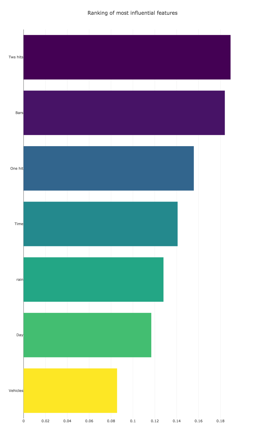
As you can see, the ranking order is quite different to the last one. The difference here is that a sample of only 1,000 accidents was used instead of the 18,000 accidents that were in the initial dataset. Even though I took a randomised sample of instances, there are big discrepancies in the data. According to this sample dataset, the number of bars in the area is the biggest determining factor in an accident, quite a bit more than the weather. It would be nice to have weather data for all samples in the dataset, but either you would need to upgrade to a paid membership on DarkSky.net to get more calls, or you would need to 3600 second sleeps between each batch of API calls, which would amount to more than 18 hours waiting.
Creating a Google Maps plot of the accidents
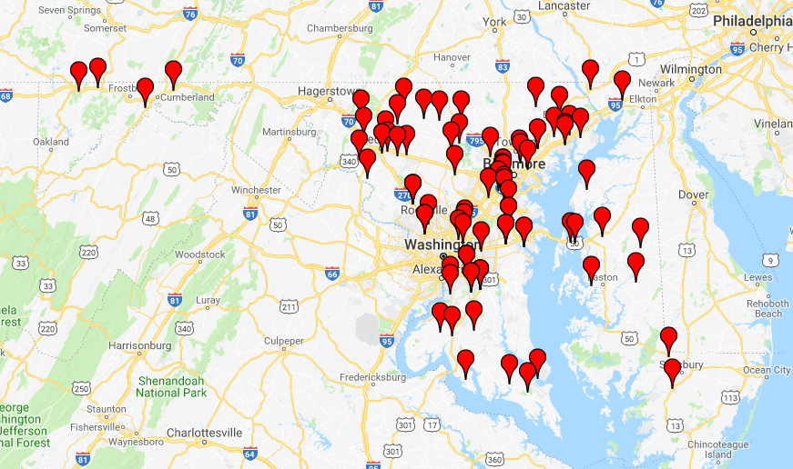
I will now obtain the latitude and longitudes of the nearest intersections of 100 accidents and plot them on a Google map, using the Google Map Plotter.
crash_plot_df = data_sample_geo_df.sample(n=100, random_state=0)
crash_plot_df['intersection'] = crash_plot_df['ROAD'] + ' ' + crash_plot_df['INTERSECT_ROAD'] + ' ' + crash_plot_df['COUNTY_NAME'] + ' ' + 'MARYLAND'
# TMakes calls to the gmaps API to get latitude information for an address
def get_lat(x):
    try:
        return gmaps.geocode(x)[0]['geometry']['location']['lat']
    except:
        return ''

# Makes calls to the gmaps API to get longitute information for an address
def get_lng(x):
    try:
        return gmaps.geocode(x)[0]['geometry']['location']['lng']
    except:
        return ''

# Lat and lon info is then added to the dataframe
crash_plot_df['crash_lat'] = crash_plot_df['intersection'].apply(get_lat)
crash_plot_df['crash_lng'] = crash_plot_df['intersection'].apply(get_lng)
Finally, I will plot all of the points and use the gmplot API to create an HTML file with a map of Maryland and the crash sites.
from gmplot import gmplot

# Coordinates for Maryland
state_lat = gmaps.geocode('Maryland')[0]['geometry']['location']['lat']
state_lng = gmaps.geocode('Maryland')[0]['geometry']['location']['lng']

# Place map
gmap = gmplot.GoogleMapPlotter(state_lat, state_lng, 8)

# Coordinates for Counties
county_lats = crash_plot_df['lat'].values.tolist()
county_lngs = crash_plot_df['lng'].values.tolist()

# Coordinates for crashes
crash_lats = crash_plot_df['crash_lat'].values.tolist()
crash_lngs = crash_plot_df['crash_lng'].values.tolist()

# Scatter points
gmap.scatter(crash_lats, crash_lngs, 'red', size=2500, marker=True)

# Draw
gmap.draw("my_map.html")
Here is what you will see when you open up the HTML file.