Time-series Prediction using XGBoost

Introduction

XGBoost is a powerful and versatile tool, which has enabled many Kaggle competition participants to achieve winning scores. How well does XGBoost perform when used to predict future values of a time-series? This was put to the test by aggregating datasets containing time-series from three Kaggle competitions. Random samples were extracted from each time-series, with lags of t-10 and a target value (forecast horizon) of t+5. Up until now, the results have been interesting and warrant further work.

Data loading and preparation

All datasets were obtained from Kaggle competitions.

Wikipedia views data

Web Traffic Time Series Forecasting: https://www.kaggle.com/c/web-traffic-time-series-forecasting

Time-series data from 1000 pages used.

Supermarkets sales data

Corporación Favorita Grocery Sales Forecasting: https://www.kaggle.com/c/favorita-grocery-sales-forecasting

Time-series data for 1000 items used.

Restaurant vistors data

Recruit Restaurant Visitor Forecasting: https://www.kaggle.com/c/recruit-restaurant-visitor-forecasting

Time-series data for 100 restaurant outlets used.

Concatenating all datasets into one dataset

Time-series from each dataset have varying periods, so the input creation class is called separately for each dataset in order to create training sets for supervised learning. Once training sets have been created, they are concatenated into one X-matrix and with a corresponding y-vector containing the target variables.

Classes

I created the following class in order to convert each time-series into a specified number of samples, which could then be used in a supervised learning context. The number of steps in each sample represents the lag (t-n) up until the last step, which is the current time (t). A forecast horizon (t+n) is selected for each sample and becomes the corresponding target value. For each example, a lag of ten steps was used and a forecast horizon of five steps in the future was used. Five steps produced better results than one step, three steps and ten steps.

class create_inputs:
    def __init__(self, sample_num, lag, lead):
        self.sample_num = sample_num
        self.lag = lag
        self.lead = lead

    def fit(self, X, y=None):
        self.X = X

    # X must be an numpy matrix or array
    def transform(self, X, y=None):
        X_matrix = []
        y = []

        for row in range(len(X)):

            ts = self.X[row]

            for i in range(self.sample_num):
                np.random.seed(i)
                start_point = np.random.randint(1, len(ts) - self.lag - self.lead)

                sample = []
                for n in range(self.lag + 1):
                    sample.append(ts[start_point + n])

                X_matrix.append(sample)
                y.append(ts[start_point + self.lag + self.lead])

        self.X = np.array(X_matrix)
        self.y = np.array(y)
        return self.X, self.y

    def fit_transform(self, X, y=None):
        self.fit(X)
        return self.transform(X, y=None)

Configuring optimal XGBoost model

A grid search was conducted that tried various values for:

• The number of trees in the forest
• Maximum depth of all trees in forest
• The learning rate

The grid search settled for 20 trees, each with a maximum depth of 10 and learning rate of 0.1.

Making predictions using randomly selected time-series

Six time-series are used from each dataset, which were put aside in the beginning for the purpose of testing.

In order predict in a walk-through manner - that is, predict each step in the series sequentially - the following function was used to create a stack of test examples that progress sequentially.

def timeseries_to_supervised(data, lag=1, lead=1):
    df = pd.DataFrame(data)
    columns = [df.shift(-i) for i in range(0, lag+1)]
    df_X = pd.concat(columns, axis=1)
    df_all = pd.concat([df_X, df.shift(-(lead + lag))], axis=1)
    df_all = df_all.iloc[:-(lead + lag), :]
    df_all.fillna(0, inplace=True)
    return df_all

Results

The predictions for each of the six examples from each dataset were plotted on top of the original time-series to visually compare the model’s predictive power in each case. The blue curves are the original time-series and the orange curves are the predicted values. A period of three months was chosen for all examples.

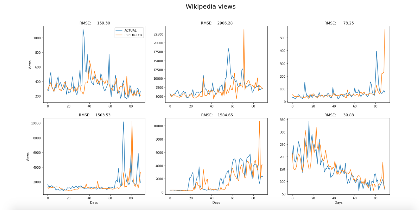
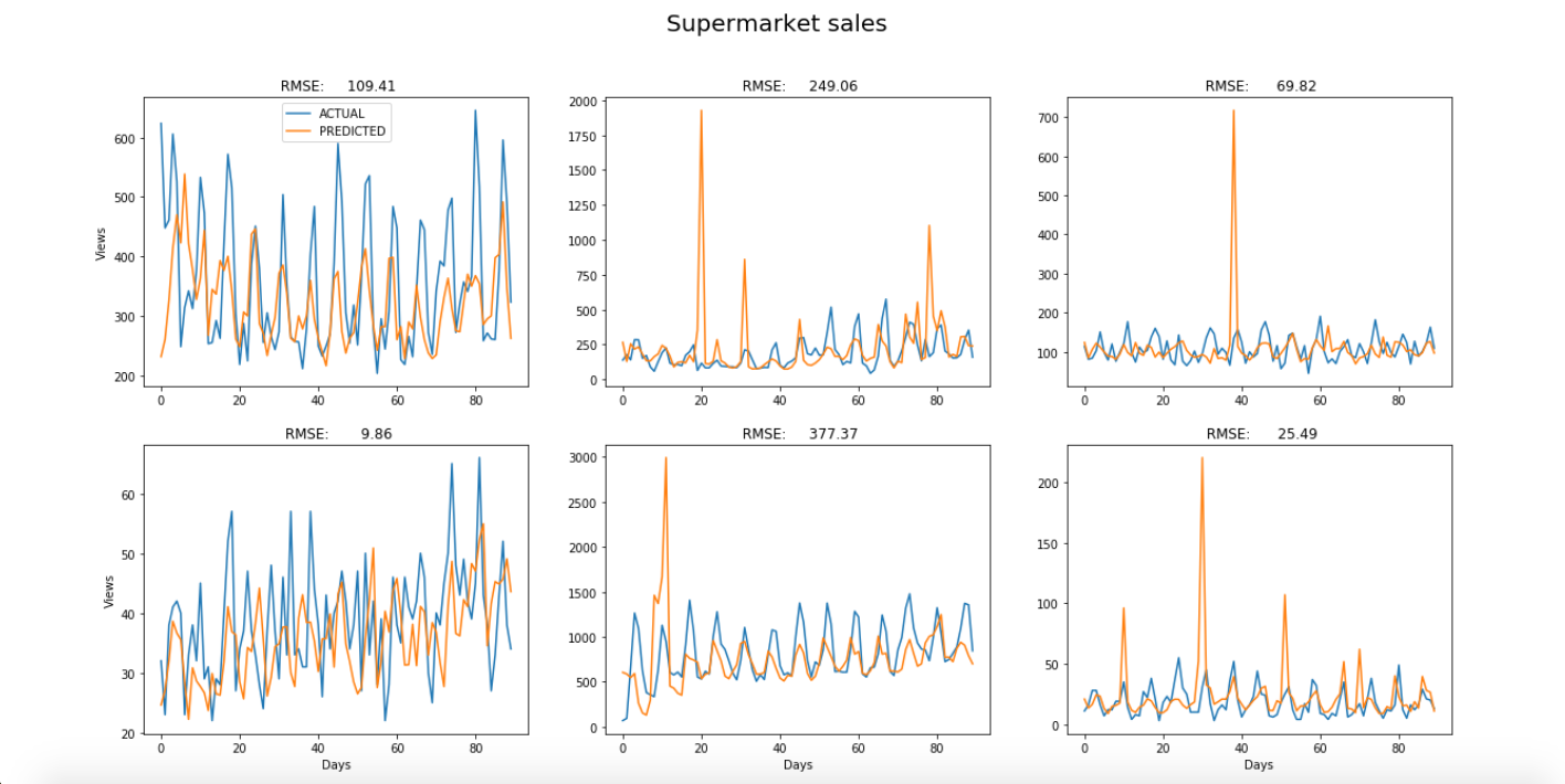
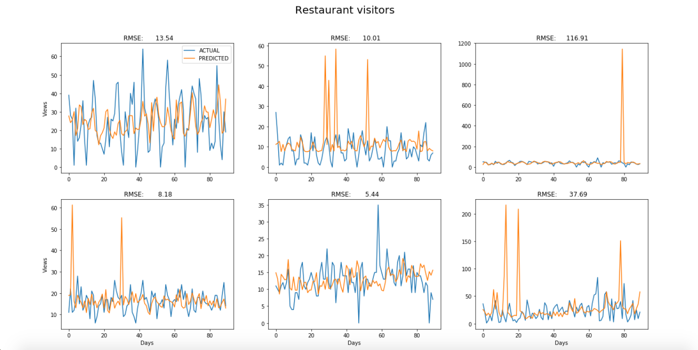
As you can see, the results are especially good when the model is used to predict supermarket sales, which have relatively stable trends and seasonality, and appear to have less noise. About half of the graphs show that the model spikes significantly in places. This might be rectified by increasing the number of examples used to train the model.